Common Questions in Analytics Interviews - Part 2 | Statistics Basics
- Dec 9, 2025
- 4 min read
This is the Part-2 of our article series on Common Questions in Analytics Interviews.
Part-1 focuses on common questions related to SQL.
In this article, we focus on Basics of Statistics.
Machine Learning, Artificial Intelligence etc.... the basis of all this is Statistics. So, if you are interested in Analytics, learning Statistics should be on the top of your list!
What are metrics of Central Tendency?
Metrics of Central Tendency are numbers used to describe the centre of a dataset.
Datapoints = [4, 6, 10, 20, 20]Mean (Average)
This is the simplest of the metrics. It is the sum of all datapoints divided by the count of data points.
Mean = (4 + 6 + 10 + 20 + 20) / 5
Mean = 12
Pros
Very easy to compute
Easy to comprehend
Can summarise the dataset well (except in the case of outliers)
Cons
Does not work well with outliers. (A single very high value can push the mean up)
Does not provide any insight into the distribution of datapoints.
Median
This is the midpoint when all the datapoints are arranged in an ascending order.
Datapoints = [4, 6, 10, 20, 20]
Median = 10
Pros
Gives insight into the distribution of the datapoints
50% points are above the median and 50% are below
Not skewed even if outlier are present
Cons
Computationally intensive (as first the series needs to be sorted)
Mode
This is the most common datapoint in a dataset
Datapoints = [4, 6, 10, 20, 20]
mode = 20
Pros
Can summarise categorical data (datapoints which cannot be added)
Cons
Does not provide any insight into distribution.
May not be representative of whole population.
Explain Standard Deviation
Wikipedia defines Standard Deviation (SD) as
In statistics, the standard deviation is a measure of the amount of variation of the values of a variable about its mean.
In short, it tells us how varied our dataset is. SD is calculated as

Calculate the Mean of the dataset
Calculate the difference between every datapoint and the mean
Square each difference, and sum up the square of differences
Divide the variance by count of datapoints (this is called Variance)
Take Square Root of Variance
Let's understand this with an example
Datapoints = [4, 6, 10, 20, 20]

Calculating the Mean
Mean = (4 + 6 + 10 + 20 + 20) / 5
Mean = 12


Adding up the square of differences with each datapoint and mean
diff = (4-12)^2 + (6-12)^2 + (10-12)^2 + (20-12)^2 + (20-12)^2
diff = 232


Dividing by Count of datapoints
variance = 232 / 5
variance = 46.4


Taking Square Root of Variance

SD = 6.8
Higher the SD, more spread out the data from it's mean. In this case, mean may not be a very strong metric for population summary.
Lower the SD, the data is closer to the mean. In this case, mean is a good representation of population summary
What is a Probability Distribution Function? Give some examples of common distributions
Probability Distribution Function (PDF) is a statistical function that describes the likelihood of a variable taking a specific value
Let's take an example of an unbiased dice. The probability of getting either of the 6 numbers is 16.7%. This is one of the PDFs know as Discrete Uniform Distribution.

Some of the common PDFs are
Uniform Distribution
Normal Distribution
Poisson Distribution
Binomial Distribution
What is a Normal Distribution
This is the most common distribution used in statistics.
Normal Distribution, also known as Bell Curve, is a Continuous Probability Distribution which is centred around its mean and tapers off symmetrically in both directions
Let's take an example. Assume we have to plot the histogram of weight of every person in our country. When we plot it, what we'll observe is
Majority of the people are centred around a particular value (e.g. 70kgs)
As we go higher / lower, the no. of people with that weight will reduce.
There will be very few extreme cases (e.g. 120+kgs or < 30kgs)
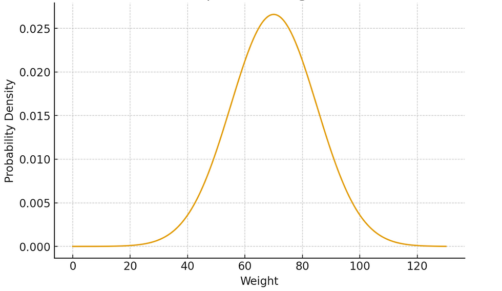
A special case of such a curve is Normal Distribution which is represented by the following formula

x is the weight
f(x) is the Probability of a particular weight
What is Skew and Kurtosis?
Skew and Kurtosis - both the concepts are related to the shape of probability distributions.
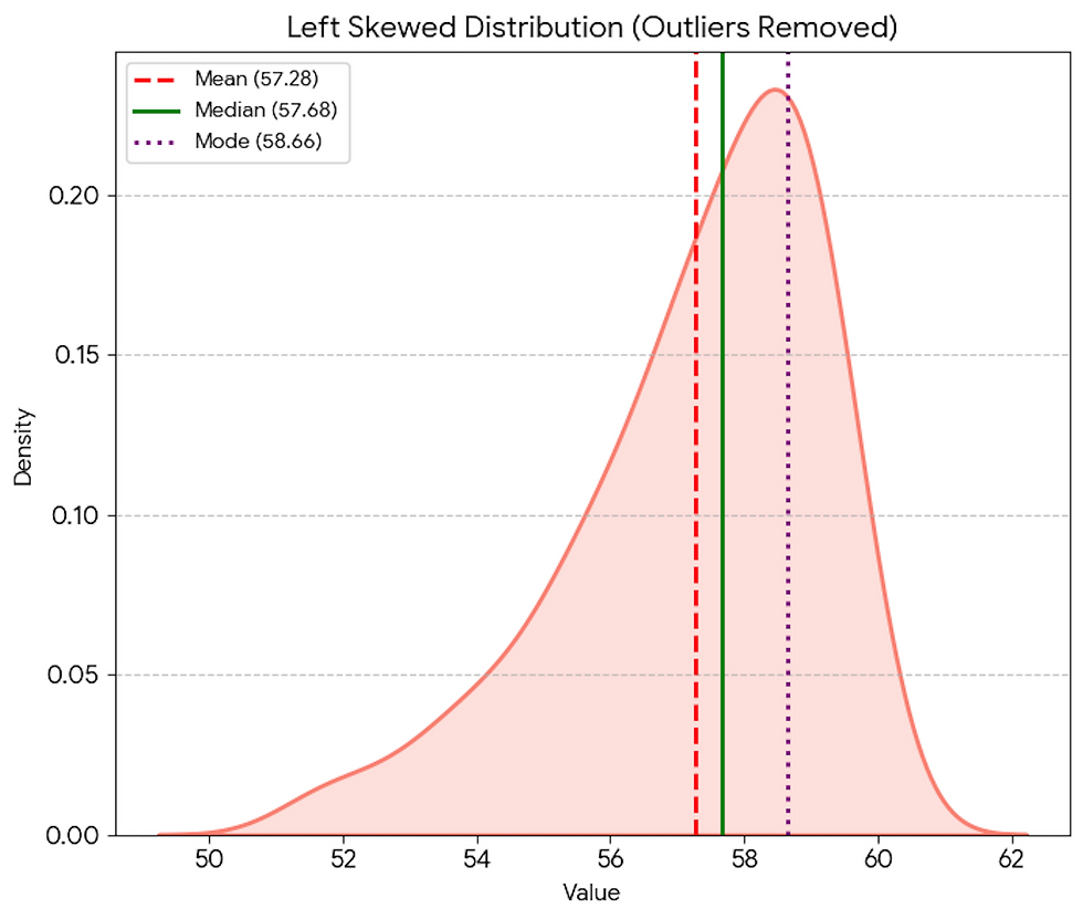
Skew refers to the asymmetry of the distribution.
Left Skew
Left skewed distribution has more outliers on the left side of the mean
Mean < Median
Right Skew
Right skewed distribution has more outliers on the right side of the mean
Mean > Median

Kurtosis refers to how heavy the tails and how peaked the distribution is.
Distribution with higher peak has thinner tails (since area under the curve is constant)
Distribution with lower peak has thicker tails.

And that's it.
The concepts of statistics are far from over. And I'll publish many more articles regarding statistical concepts. But these few concepts mentioned above are the basics of everything and knowing these is crucial for any Analyst.
Until next time!

Comments