Common Questions in Analytics Interviews - Part 3 | Spreadsheets
- Dec 23, 2025
- 5 min read
This is the Part-3 of our article series on Common Questions in Analytics Interviews.
Previous part explains the Basics of Statistics
In this part we talk about one of the most crucial tools for an Analyst - Spreadsheets. Even today, majority of the analyses and reporting happens on Spreadsheets, mainly because they are very simple to understand and yet so powerful.
The most common spreadsheet tools used are
Microsoft Excel
Google Sheets
In this article, we focus on Google Sheets (majority of the functionality is very similar in both the tools. So, if you're familiar with one, the other is very easy to learn)
What are Aggregation Functions?
These functions are the basics of Spreadsheets.
SUM: Adds up the numbers in the selected Cells
AVG: Calculates the Average of numbers in selected Cells
COUNT: Counts the cells in which there is some data
The following image shows how to calculate the sum of the Total Revenue of the table in a spreadsheet.
In a cell, start by typing "=". This shows all the functions available in the spreadsheet.
Enter "=SUM" and hit Tab button. Now, the function allows us to select the cells that we want to add
We can manually select the cells with our pointer, or we can type C2:C12
This formula basically says, add up all the values in cells C2:C12 and paste then sum in the cell.
Similar steps are followed for any other aggregate functions.

What are Conditional Aggregation Functions?
In the above example, we added the Revenue for all the Dates for all the Countries. But, what is we only wanted to add the revenue from India?
This is where Conditional Aggregate Functions are used. Basic functions are
SUMIF (or SUMIFS)
COUNTIF (or COUNTIFS)
AVERAGEIF (or AVERAGEIFS)
These functions take in multiple arguments.
The Range of cells which we want to aggregate
The Range of cells on which we want to apply a condition
The value of the Condition
The following image shows the formula for Adding Revenue of India only

The function used here is SUMIF()
First argument of the function is B2:B12. (the cells on which the filtering conditions needs to be applied)
Second argument is "India" (the value of the condition)
Third argument is C2:C12 (the cells that we want to aggregate)
What this function does is
Using First and Second arguments, filters out the rows which have India as the Country
After such rows are filtered out, adds up the revenue of only those rows.
This is how the SUMIF() function works. An extension of this is the SUMIFS() function. The only difference is that SUMIF() takes only 1 condition, while SUMIFS() can take multiple conditions (e.g. Total Revenue from India in the month of January)
What are Lookup Functions?
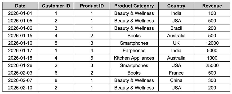
In the above examples, we worked on data which was available in a single table. But, the actual data is never available in such a clean format. Following is a very simplistic example of how data is stored in multiple tables.
Data is stored in 2 separate tables.
Table 1 has Transaction details for every customer
Table 2 has the Country mapping of every customer

Now, if we want to get the total revenue from India
First, we need to map the country of each user in Table 1 using Table 2
Then we can use the SUMIF() function as mentioned above.
How can we map the Country for each user in Table 1?
This is where Lookup functions become crucial. There are mainly 2 lookup functions
VLOOKUP()
HLOOKUP()
Let's understand the VLOOKUP() function. As the name suggests it is a Vertical-Lookup function.
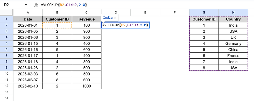
There are 4 inputs to the VLOOKUP() function
B2 - the value that we want to lookup
(We want to get the country of Customer ID = 1 )
G1:H9 - the table from which we want to fetch the data
(this is the Table 2 which has the Customer<>Country Mapping. This
The column number in Table 2 in which our expected values are present
(the Country is present in Column 2 of the Table 2)
This is an optional argument. It tells the function whether the Table 2 is sorted or not. It becomes important when there are multiple mappings present for out Lookup key. (if there are multiple country mappings present for Customer ID = 1, this argument becomes important)
To explain it simply, the function
looks up the value in B1
Filters the rows in Table 2 which has Column 1 value = value in B1
Gets the value in 2nd column of Table 2 for the filtered row
Pastes the value in our cell.
This is how we can easily get the mapping for all the Customers.
Note: The column which we want to search on i.e. Customer ID should alway be the First Column in Table 2. Otherwise, VLOOKUP() cannot fetch the values.
HLOOKUP() does the same thing but for when we want to search for values in columns, instead of rows.
What are Pivot Tables?
Pivot Tables are the basis of all the Business Intelligence tools. All the BI tools like Tableau, Power-BI, under the hood, operate very similar to how Pivot Tables operate. Once we understand Pivot Tables, it is easy to pick up and master any of these tools.
Let's understand with an example. Following is a sample table which captures revenue.
What if we want to summarise this dataset in different ways?
What is the Revenue from India?
How much revenue is received from Books category?
How many Customers purchased from USA?
What is the Revenue per User from Australia?
What is the Avg. Revenue per User in Smartphones category?
We can definitely use the formulae that we discussed before (SUM, SUMIFS, COUNTIFS etc). But is there a simpler way which allows us to apply multiple conditions? Multiple aggrgations?
Enter Pivot Tables!
To create a pivot table
Select all the data in the table
Go to Insert and click on Pivot Table

This will create another sheet as shown below

We can see following things in the Pivot Table Editor
Rows
Columns
Values
Filter
All columns present in out Raw Table
Now, let's populate data into the table!
Select Country in Rows
Select Product Category in Columns
Select Revenue in Values
.... and we get a beautiful table as shown below.
It shows the Revenue per Country. Also shows Revenue per Category. Along with that, we also get the Country + Category Breakdown!
1500 is the total Revenue from Australia
500 in from Books and 1000 is from Kitchen Appliances
In short, every single Cell in the Table is a SUMIFS() function with condition on Country and Product Category. But, instead of creating multiple formulae, this Pivot Table is able to show multiple calculations with only a few clicks!

If we want, we can add additional metrics in the Values field, we can add Date filter in the Filters etc.
You can imagine how powerful this tool is for Reporting or carrying out some exploratory analysis
And that's all for this article. There obviously are many more functionalities in the Spreadsheet, but the functions mentioned above form the vary basics of understanding spreadsheets!
We'll definitely have more articles regarding more complex functions in a spreadsheet and their use-cases.
Until then...keep learning!


Comments